
In millimetric applications, an oscillator is a common module in many analogue circuits. The following article offers some suggestions of how to model the piezoelectric resonator that is its principal component.
The RLC circuit representing the impedance of a crystal resonator is shown by a two-terminal equivalent in figure 1.
 |
The circuit above shows, the static capacitance C0, representing the effect of an insulator separated by two electrodes, and the motional branch L1-C1-R1 is an equivalent to an isolated mode of piezoelectric vibration, simulating inertia, restoring force and friction respectively. Devices in a metal can may need to be modelled by a three terminal equivalent that includes the capacitance of the holder, see figure 2. If necessary, other unwanted oscillation modes such as spurs may be simulated as additional motional branches in parallel with L1-C1-R1.
Accurate calculation of the component values in the equivalent circuit is vital to give a reliable simulation. Loading the standard model, usually for a 10MHz crystal, will produce the wrong frequency for parallel or series resonant modes: also, in a pulling circuit, incorrect values of motional capacitance will give an erroneous sensitivity to a varying load capacitance.
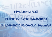
Taking, as example, a 27MHz fundamental crystal with a load capacitance of 12pF and pulling sensitivity of 20ppm/pF. The equation of motional resonance is Fs = 1/ [2??(L1 * C1)]
For parallel resonance Fp = Fs[1 + C1/(2*C0)] = 27.000MHz
For pulling sensitivity S = 1000000 * C1/ 2(C0 + Cl)² = 20ppm/pF
Where CL, the load capacitance, is 12pF. If we specify C0, as a shunt capacitance of 3pF, then the motional capacitance C1 is 9pF, Fs becomes 26.95956MHz and the motional inductance L1 is 3.87mH. A reasonable range of values for motional resistance would be 20? for a 30MHz crystal and 60? for a 10MHz. For other frequencies:
| Frequency (MHz) | R1 (Ohms) | L1(mH) | C1 (pF) | C0 (pF) |
| 2.00 | 200 | 520 | 0.012 | 4 |
| 5.00 | 50 | 115 | 0.010 | 3 |
| 15.00 | 30 | 12.5 | 0.009 | 5 |
| 30.00 | 20 | 4.7 | 0.006 | 3 |
Simulation of a ceramic resonator is more difficult, as these three terminal parts contain internal load capacitors, and the ratio of reactance to impedance is lower than the value for crystals. The resonance frequency is also lower than that for a crystal, so the size of the reactive components is further reduced. This reduction in the Quality Factor means a faster start-up but the drawback is that load capacitor values have a greater influence on oscillator frequency than with a crystal.
Typical values for two terminal resonators are:
| Frequency (MHz) | R1 (Ohms) | L1(mH) | C1 (pF) | C0 (pF) |
| 3.58 | 7 | 0.113 | 1936 | 140 |
| 6.0 | 8 | 0.094 | 8.3 | 60 |
| 8.0 | 7 | 0.092 | 4.6 | 40 |
| 11.0 | 10 | 0.057 | 3.9 | 30 |
Modelling the start-up of any oscillator is also a difficult exercise. The Barkhausen criteria are: loop gain in the oscillator has to be equal to or greater than unity, and phase shift must be a multiple of 2 ?, for the circuit to start. In practice, the addition of a large resistor in parallel with crystals or resonators improves the starting, so a resistor value of 1Megohm across resonators, 10Megohm across crystals running above 1MHz, and 22Megohm across watch crystals is likely to get some positive results in a simulation too.